set SRC1=toes.png
WTF is a Kurtosis?
Measures of the colours in channels of an image.
IM can calculate statistics for each channel: minimum, maximum, mean, median, standard deviation, skewness, kurtosis and entropy. These statistics depend only on values in the channel, and are independent of the position of those values. If we shuffled the pixels, the result would have the same statistics.
%IMG7%magick toes.png -colorspace Gray -verbose info: | grep -A 10 statistics:
 Channel statistics:
    Pixels: 62211
    Gray:
      min: 6050.94  (0.0923314)
      max: 60401.1 (0.921662)
      mean: 32313.7 (0.493075)
      median: 31438.8 (0.479725)
      standard deviation: 9476.19 (0.144597)
      kurtosis: 0.171096
      skewness: 0.172407
      entropy: 0.980554
All of these except entropy are available in %[fx:...] expressions.
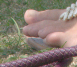
We will use the usual toes image.
set SRC1=toes.png |

|
This is also called the arithmetic mean or average. The mean is the sum of the values, divided by the number of values. It is often notated as μ or !`mu!` (mu) or x̄ or !`bar x!` (x-bar).
!`mu = (1/n) * sum_(i=1)^n x_i !`
The mean is always within the range of the minimum and maximum values:
!`min_(i=1)^n(x_i) <= mu <= max_(i=1)^n(x_i)!`
The expected value is a more general concept: it is a weighted mean, the average of possible values each weighted by its probability.
If we repeatedly pick the value of a channel from a random pixel, and calculate the arithmetic mean of the values picked so far, that mean will approach the expected value of that channel in the entire image.
Here, we give pixel values as a percentage of QuantumRange, but the result of "-format %[fx:...]" is a proportion of QuantumRange:
%IMG7%magick xc:gray(10%%) xc:gray(20%%) xc:gray(30%%) xc:gray(40%%) ^
  +append +repage ^
  -format %%[fx:mean] ^
  info:
0.25
For the toes image:
%IMG7%magick %SRC1% ^
  -format %%[fx:mean] ^
  info:
0.488162
This is the "half-way" value. In general, the median is defined as any value such that at least half the population is less than or equal to that value, and at least half the population is greater than or equal to that value. In that definition, when there is an even number of values, there is no unique median; it may take a number of values.
Commonly, when there is an even number of values, the median is taken to be the arithmetic mean of the central two values.
IM uses a different definition for an even number of values: it uses the lower of the two central values. So IM's median value will always be one of the values from the image.
An odd number of values:
%IMG7%magick xc:gray(10%%) xc:gray(20%%) xc:gray(30%%) xc:gray(40%%)  xc:gray(50%%) ^
  +append +repage ^
  -format %%[fx:median] ^
  info:
0.3
An even number of values:
%IMG7%magick xc:gray(10%%) xc:gray(20%%) xc:gray(30%%) xc:gray(40%%) ^
  +append +repage ^
  -format %%[fx:median] ^
  info:
0.2
An odd number of colour values:
%IMG7%magick xc:sRGB(5%%,25%%,30%%) xc:sRGB(15%%,30%%,40%%) xc:sRGB(30%%,20%%,5%%) ^
  +append +repage ^
  -verbose info: |grep -i median
 median: 9830.25 (0.15)
      median: 16383.8 (0.25)
      median: 19660.5 (0.3)
      median: 15291.5 (0.233333)
The output has median values for each of the red, green and blue channels, and the composite result which is the arithmetic mean of the other medians.
We can use "%[fx:meadian]" to get just one channel median, or the composite result:
%IMG7%magick xc:sRGB(5%%,25%%,30%%) xc:sRGB(15%%,30%%,40%%) xc:sRGB(30%%,20%%,5%%) ^
  +append +repage ^
  -format %%[fx:median] ^
  info:
0.233333
For the toes image:
%IMG7%magick %SRC1% ^
  -format %%[fx:median] ^
  info:
0.472964
This is a measure of how much the values vary from the mean. For an image, it is a measure of contrast.
The lower bound is zero, when there is no variation, no contrast.
The units of mean and standard deviation are the same as the units of the thing measured. (Skewness and kurtosis have no units.)
The SD is the square root of the variance, where the variance is the mean of the squares of the values minus the square of the mean.
!`variance = 1/n * sum_(i=1)^n(x_i^2) - mu^2 !`
!`sigma = sqrt(variance) !`
... where n is the number of values.
However, when used as an algorithm (sometimes called the "textbook" algorithm), this is numerically unstable. The two numbers that are subtracted can be very much larger than their difference, so the difference is swamped by imprecision. The result of the subtraction is inaccurate and can be negative, resulting in NaN (Not a Number) from the square root. An alternative definition of variance, that is stable when used as an algorithm, is:
!`variance = 1/n * sum_(i=1)^n((x_i-mu)^2) !`
We might calculate the SD of an entire population. Or we might calculate the SD of some samples from a population, in which case we might assume this is an estimate of the SD of the entire population. This uncorrected sample standard deviation, when it is calculated using the mean of the samples, is a biased estimator: it is usually too low, so we might adjust ("correct") this number to obtain a better ("unbiased") estimate.
The upper bound of the SD of a population, or of an uncorrected sample SD, is half the upper bound of the population values.
The usual correction is to calculate the variance dividing by !`(n-1)!` instead of !`n!`. This is Bessel's correction.
!`variance = 1/(n-1) * sum_(i=1)^n((x_i-mu)^2) !`
... where !`n!` is the number of samples.
The unbiased sample variance !`s^2!` and the biased sample variance !`s_n^2!` are related by:
!`s^2 = n/(n-1) * s_n^2 !`
The standard deviation may be notated as SD or !`sigma!` or σ (sigma) or s. Beware that any of these might refer to the standard deviation of the entire population, or of a sample, or a biased estimate for the entire population, or of an unbiased estimate for the entire population. An estimate is sometimes notated with a "hat": x̂ or !`hat x!` (x-hat) or σ̂ (sigma-hat).
IM calculates SD from the unbiased sample variance, as we can demonstrate:
%IMG7%magick ^
  xc:Black xc:White ^
  +append +repage ^
  -format %%[fx:standard_deviation] ^
  info:
0.707107
For the toes image:
%IMG7%magick %SRC1% ^
  -format %%[fx:standard_deviation] ^
  info:
0.153221
Skewness is a dimensionless signed number that measures symmetry. IM calculates skewness from moments. Other definitions of skewness are available.
A symmetrical distribution has zero skewness.
In a positive skew, values on the right of the mode are spread over a greater range than the values on the left.
In a negative skew, values on the left of the mode are spread over a greater range than the values on the right.
It is sometimes said that positive skew implies that mode < median < mean, and negative skew implies that mean < median < mode. But counter-examples are easily created:
For convenience, we will set an environment variable for writing some statistics:
set sFMT=^
mean=%%[fx:mean] ^
SD=%%[fx:standard_deviation]\n^
skew=%%[fx:skewness*QuantumRange] ^
kurt=%%[fx:kurtosis*QuantumRange]\n
|
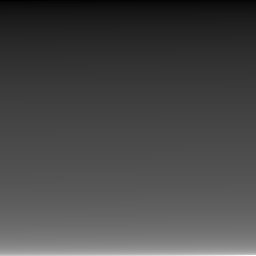
Create an image with
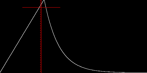
shark-fin distribution,
set Pk=0.3

%IM7DEV%magick ^
  -size 1x65536 gradient: -colorspace Gray -rotate 90 ^
  -fx "u<%Pk% ? u/%Pk% : exp(-(u-%Pk%)*10)" ^
  -process 'cumulhisto norm verbose' ^
  -process 'invclut' ^
  -crop 256x +repage -append +repage ^
  +write chst_shkfin.png ^
  -format "%sFMT%" ^
  info:

call %PICTBAT%histoGraph ^
  chst_shkfin.png chst_shkfin_hg.png
mean=0.27970417 SD=0.12791226 skew=3.2649812e+09 kurt=6.5086751e+09 |
|
The image has a positive skew, and median < mean < mode.
The Pearson coefficient of skewness (see https://gacbe.ac.in/pdf/ematerial/18BST13C-U4.pdf) is defined as either:
!`(mu-text(mode))/sigma!`
... or as ...
!`3*(mu-text(median))/sigma!`
... where !`mu!` is the mean and !`sigma!` is the standard deviation.
In Bowley's coefficient of skewness, we define Q1 such that 25% of the values are below Q1; M (the median) such that 50% of the values are below M; Q3 such that 25% of the values are above Q3. Then the skewness is:
!`(Q_3+Q_1-2*M)/(Q_3-Q_1) !`
The skewness can be defined in terms of central moments. There are two related forms: !`beta_1!` (beta-one) and !`gamma_1!` (gamma-one).
!`beta_1 = (mu_3)^2 / (mu_2)^3 !`
... or ...
!`gamma_1 = sqrt(beta_1) !`
!`\ \ = mu_3 / (mu_2)^(3//2) !`
The last of these is the definition used by IM. This is also called the third standardized moment.
The algorithm IM previously used to calculate skewness was the "textbook" method:
skewness = ( sum_cubed/area
             - 3*mean*sum_squared/area
             + 2*mean*mean*mean
           ) * 1/(SD*SD*SD)
For the toes image:
%IMG7%magick %SRC1% ^
  -format "%%[fx:skewness * QuantumRange]" ^
  info:
0.364843
Kurtosis is a measure of the outliers.
IM calculates the excess kurtosis, which is the non-excess kurtosis minus three. The non-excess kurtosis is sometimes called Pearson's kurtosis or simply kurtosis. Beware of the confusing terminology.
Pearson's kurtosis has a minimum value of the squared skewness plus one. It has no upper limit.
A normal distribution has an excess kurtosis of zero, which is called mesokurtic.
A distribution with positive excess kurtosis is called leptokurtic.
A distribution with negative excess kurtosis is called platykurtic.
The non-excess kurtosis !`kappa!` (kappa) is:
!`kappa = mu_4 / sigma^4 !`
... where μ4 is the fourth central moment, and σ is the standard deviation.
The old way IM calculated kurtosis (strictly speaking, "excess kurtosis") was by the "textbook" method:
kurtosis = ( sum_fourth_power/area
             - 4.0 * mean * sum_cubed/area
             + 6.0 * mean * mean * sum_squared/area
             - 3.0 * mean * mean * 1.0 * mean * mean
           ) * 1 / (SD*SD*SD*SD)
           - 3.0;
Why did the mutliplication of the means include a multiplication by 1.0? I don't know.
For the toes image:
%IMG7%magick %SRC1% ^
  -format "%%[fx:kurtosis * QuantumRange]" ^
  info:
0.0394962
A moment is, loosely speaking, the sum of the signed distances of values from a central value. The signed distances may be raised to a power. Moments can be raw or central. Central moments can be standardized.
Raw moments are moments about zero. The kth raw moment is the expected value of xk:
!`mu'_k = bb "E"[x^k] !`
The expected value of x is sometimes notated as <x> or !`(:x:)!`.
Central moments are moments about the mean. Standardized moments are raw moments divided by the appropriate power of the standard deviation.
The general kth moment can be defined, where k is any real number. But the moments for k=1, k=2, k=3 and k=4 are particularly useful. When k is an even number (2, 4, 6...), the moment is non-negative.
For some infinite distributions, some moments may be undefined. For example, the (infinite) Cauchy distribution has fractional central moments, but no moments greater than or equal to one. Hence it has no mean, variance or standard deviation.
The first raw moment is:
!`mu'_1 = 1/n * sum_(i=1)^n(x_i) !`
The first raw moment is the arithmetic mean.
The kth raw moment is:
!`mu'_k = 1/n * sum_(i=1)^n((x_i)^k) !`
Central moments are moments about the mean, instead of zero. The first central moment is:
!`mu_1 = 1/n * sum_(i=1)^n(x_i-mu) !`
The kth central moment is:
!`mu_k = 1/n * sum_(i=1)^n((x_i-mu)^k) !`
The second central moment is the variance.
The raw and central moments can be calculated from each other (see the Wolfram references):
μ1 = 0
μ2 = μ'2 - μ'12
μ3 = μ'3 - 3μ'2μ'1 + 2μ'13
μ4 = μ'4 - 4μ'3μ'1 + 6μ'2μ'12 - 3μ'14

μ'1 = arithmetic mean
μ'2 = μ2 + μ'12
μ'3 = μ3 + 3μ2μ'1 + μ'13
μ'4 = μ4 + 4μ3μ'1 + 6μ2μ'12 + μ'14
Standardized moments are calculated from central moments and the standard deviation. The kth standardized (aka "normalized") moment:
= μk
  σk
Standardized moments are dimensionless quantities; they have no units.
The standardized third central moment is the skewness, !`gamma!` (gamma).
The standardized fourth central moment is the kurtosis (aka Pearson kurtosis, non-excess kurtosis), κ (kappa).
(a+b)2 = a2 + 2ab + b2

(a+b)3 = (a+b)*(a2 + 2ab + b2)
       = a3 + 2a2b + ab2 + a2b + 2ab2 + b3
       = a3 + 3a2b + 3ab2 + b3

(a+b)4 = (a+b)*(a3 + 3a2b + 3ab2 + b3)
       = a4 + 3a3b + 3a2b2 + ab3 + a3b + 3a2b2 + 3ab3 + b4
       = a4 + 4a3b + 6a2b2 + 4ab3 + b4

(a-b)2 = a2 - 2ab + b2

(a-b)3 = (a-b)*(a2 - 2ab + b2)
       = a3 - 2a2b + ab2 - a2b + 2ab2 - b3
       = a3 - 3a2b + 3ab2 - b3

(a-b)4 = (a-b)*(a3 - 3a2b + 3ab2 - b3)
       = a4 - 3a3b + 3a2b2 - ab3 - a3b + 3a2b2 - 3ab3 + b4
       = a4 - 4a3b + 6a2b2 - 4ab3 + b4
To calculate sum2 etc, we know the value of (a-b)2.
... nobody knows what entropy really is, so in a debate you will always have the advantage.
- John von Neumann quoted by Claude Shannon.
This measures the average level of information, aka "surprisal". What IM calls entropy is a measure of each channel from 0.0 to 1.0 of how evenly the values (rounded to 16 bits) are spread among the values that are present. If all the values in a channel are the same (only one value is present), the entropy is zero. If the values are evenly spread, the entropy is one. Aside from the rounding to 16 bits, this measure is also known as the information dimension.
Unlike the other statistics on this page, the pixel values are not directly relevant. The measurement is calculated only from probabilities. The probability of a value is the fraction of the population that have that value.
IM's measure is closely related to what the literature calls entropy, but is not the same.
From the Wikipedia reference, entropy H (aka Shannon entropy) is:
H = -sum ( p(xi) * logb(p(xi)) )
!`H = -sum_(i=1)^n(p(x_i) * log_b(p(x_i))) !`
... where !`p(x_i)!` is probability of the value !`x_i!`, in the range 0 to 1. The log is to base !`b!`.
Where does this come from?
The information content of a value increases as the probability of that value decreases. If the probability is close to 0, the IC is high. If the probability is close to 1, the IC is low. To accomplish this, the information content of one value x is:
I = -logb(p(x)) = logb(1/p(x))
Note that:
-log (A) = log (1/A)

log10(A) / log10(B) = logB(A)
One observation of a value xi carries information I(xi)=log(1/pi).
When all values are the same, so a particular value is certain, an observation of that value carries no information:
I (1) = 0
The I(xi)=log(1/pi) formula also has the property that when two observations are independent:
I (p1*p2) = I(p1) + I(p2)
In general, for N values:
I (p1*p2*...*pN) = I(p1) + I(p2) + ... + I(pN)
                 = sum (I(pi))
In N observations, assuming they are independent, we expect to see the value xi occur N*pi times. So the total information I in N observations is:
I = sum ( N*pi * log(1/pi) )
  = N * sum ( pi * log(1/pi) )
So the average information per value is:
I/N = sum ( pi * log(1/pi) )
If we have a probability distribution P = {p1,p2,...pn}, where sum(pi)=1, then the entropy of the distribution is:
H(P) = sum ( pi * log(1/pi) )
The entropy of a probability distribution is the expected value of the information of the distribution.
According to the literature, the base b is typically 2 or e (2.718...) or 10. The base determines the units of the result: bits (binary digits) or nats (natural units) or hartleys (decimal digits). Alternative names for the units are sometimes used. Sometimes the base is not given, and the units are not named. Sigh.
A different base will multiply the entropy by a factor. If entropy has been calculated with base b1, and we want it to base b2, we should multiply the entropy by log(b1) / log(b2) where those logs are to any base.
It is sometimes claimed that entropy gives a lower limit to the compressibility of data. For example, when base=2, the entropy gives the information in the data, in bits. This assumes the probability of a given value is independent of its position within the data, which is not the case for ordinary photos. For example, if the eight pixels surrounding a pixel are shades of green in an ordinary photo, the central pixel is likely to also be a shade of green.
IM calculates entropy by the following algorithm:
zeroise histogram bins

for each pixel value, increment the appropriate histogram bin

number_bins = count the bins that are not empty

entropy = 0
for each histogram entry {
  count = histogram_entry / area
  entropy += -count * log10(count) / log10(number_bins)
}
Note that:
sum (histogram_entry) = area
... so (histogram_entry / area) is the probability of a pixel falling in that bin.
log10(count) / log10(number_bins) = lognumber_binscount
In effect, the base of the logarithms is number_bins, which means entropy will be on a scale from 0.0 to 1.0.
Entropy is at a maximum when all values are equally likely. Suppose we have N bins, and the probability of a value falling in any one bin is p(xi)=1/N. From Shannon's formula for entropy:
H = -sum ( p(xi) * logb(p(xi)) )
  = -sum ( 1/N * logb(1/N) )
  = -N * ( 1/N * logb(1/N) )
  = -logb(1/N)
  = logbN
Further suppose the log base b=2, so the units of entropy are bits. Then entropy is at a maximum when:
H = log2N
For example, if N=1024 then H=log21024 = 10, which is what we should expect.
However, if we use the number of bins for the log base (as IM does), then b=N, and entropy is at a maximum when:
H = logNN = 1
So the maximum entropy as calculated by IM is 1.0, when values are evenly spread. For example:
%IMG7%magick ^
  -size 65536x1 gradient: ^
  -colorspace Gray -alpha off ^
  -verbose info: |grep entropy
entropy: 1
The minimum entropy as calculated by IM is 0.0, when all values are the same. For example:
%IMG7%magick ^
  -size 65536x1 xc:khaki ^
  -colorspace Gray -alpha off ^
  -verbose info: |grep entropy
entropy: 0
For the toes image:
%IMG7%magick %SRC1% ^
  -verbose info: |grep -i entropy
 entropy: 0.953024
      entropy: 0.944734
      entropy: 0.945023
      entropy: 0.947594
We can compare this with a 32 bit/channel floating-point image. This image is linear RGB, so we convert it to sRGB.
%IMG7%magick c:\web\im\toes_lin2.tiff ^
  -profile %ICCPROF%\sRGB.icc ^
  -verbose info: |grep -i entropy
 entropy: 0.98039
      entropy: 0.972284
      entropy: 0.980123
      entropy: 0.977599
This apparently has more entropy.
Let's make an 8 bit per channel version of the toes image, and find its entropy:
%IMG7%magick %SRC1% -depth 8 chst_toes8.png

%IMG7%magick chst_toes8.png ^
  -verbose info: |grep -i entropy
 entropy: 0.940519
      entropy: 0.908524
      entropy: 0.923026
      entropy: 0.924023
The entropy has apparently decreased, especially in the green channel, by about 5%. Sometimes it goes the other way: decreasing bit depth apparently increases the entropy. It seems to me that entropy numbers are unreliable when used on 8 bit/channel images.
From an image of 8 bits/channel, there can only be a maximum of 256 different values, so number_bins cannot be larger than 256.
Suppose we have two unique values. To get an entropy of 0.5, what are the proportions of the two values? The proportions must sum to 1.0.
number_bins = 2

entropy = 0.5 = -1/log10(2) * (p*log10(p) + (1-p)*log10(1-p))
Multiply by -log10(2):
-0.5*log10(2) = p*log10(p) + log10(1-p) - p*log10(1-p)
Rearrange to get zero on one side:
p*log10(p) + log10(1-p) - p*log10(1-p) + 0.5*log10(2) = 0 ... (1)
For what values of p is this true? There should be two solutions, symmetrically about 0.5.
We could differentiate the expression and use Newton-Raphson iteration to find p. Instead, we use solveZero.bat which needs two guesses. One solution must be between 0.0 and 0.5.
call %PICTBAT%solveZero.bat ^
  "PP*log(PP) + log(1-PP) - PP*log(1-PP) + 0.5*log(2)" ^
  chst1_ 0.0 0.5

echo PP=%chst1__PP%  Vmid=%chst1__Vmid%
PP=0.110027863644063 Vmid=7.2112055216067e-10
call %PICTBAT%solveZero.bat ^
  "PP*log(PP) + log(1-PP) - PP*log(1-PP) + 0.5*log(2)" ^
  chst2_ 0.5 1.0

echo PP=%chst2__PP%  Vmid=%chst2__Vmid%
PP=0.889972136355937 Vmid=7.21120579916246e-10
As expected, there are two solutions, and they sum to 1.0. The evaluated expressions at the solutions are both very close to zero.
We can verify the result by creating an image that contains two colours of the specified proportions of pixels. The values of the colours don't matter, so long as they are different in each channel.
%IMG7%magick ^
  -size %%[fx:floor(%chst1__PP%*10000+0.5)]x1 xc:sRGB(10%%,20%%,30%%) ^
  -size %%[fx:floor(%chst2__PP%*10000+0.5)]x1 xc:sRGB(22%%,13%%,70%%) ^
  +append +repage ^
  -verbose info: | grep entropy
 entropy: 0.499916
      entropy: 0.499916
      entropy: 0.499916
      entropy: 0.499916
As expected, entropy in each channel is roughly 0.5.
What is the entropy in a Gaussian distribution?
%IM7DEV%magick ^
  xc: ^
  -process 'mkgauss width 65536 mean 50%% sd 10%% cumul norm' ^
  -delete 0 ^
  -process 'invclut' ^
  -depth 16 ^
  +write chst_gauss_dist.png ^
  -verbose ^
  info: |grep -A 10 "Channel statistics:"
 Channel statistics:
    Pixels: 65536
    Red:
      min: 0  (0)
      max: 65535 (1)
      mean: 32767.5 (0.5)
      median: 32767 (0.49999237)
      standard deviation: 6554.9234 (0.10002172)
      kurtosis: 0.009526262
      skewness: 2.9373685e-18
      entropy: 0.98732676
The mean and SD are as requested. The skewness is virtually zero. Now we make an 8 bit/channel version, and find its statistics:
%IM7DEV%magick ^
  chst_gauss_dist.png ^
  -depth 16 ^
  -verbose ^
  info: |grep -A 10 "Channel statistics:"

goto :eof
 Channel statistics:
    Pixels: 65536
    Gray:
      min: 0  (0)
      max: 65535 (1)
      mean: 32767.5 (0.5)
      median: 32767 (0.49999237)
      standard deviation: 6554.9234 (0.10002172)
      kurtosis: 0.009526262
      skewness: 2.9373685e-18
      entropy: 0.98732676
The entropy has apparently decreased.
Raw and central moments have the same units are the values measured, raised to the appropriate power. Standardized moments have no units.
Suppose we measure the height of some people in inches. The minimum, maximum, mean and median of these numbers will obviously also be in inches. Perhaps less obviously, the standard deviation will also be in inches.
From a formula for skewness above:
γ1 =  μ3
     μ23/2
where the units of μ3 are inches cubed, and the units of μ2 are inches squared, so the units of μ23/2 are inches cubed. So the numerator and denominator are both inches cubed, so they have the same units, so γ1 has no units. It is unitless, and its value does not depend on the units of the measured heights.
A similar argument applies to kurtosis: it has no units.
If we convert the heights to centimetres, the raw numbers will be multiplied by 2.54, so the minimum, maximum, mean, median and standard deviation will also be multiplied by 2.54, and their units will be centimetres. But the values of skewness and kurtosis will not change.
The composite minimum and maximum values are set to the minimum and maximum values of all the channels.
The composite mean, standard deviation, skewness and kurtosis are set to the means of the statistics of the channels. For example, the standard deviation of the channels are added together, and divided by the number of channels.
For the composite skewness and kurtosis, this returns different values to the old code, which seemed wrong to me. When the colour channels have almost the same distribution, so the channels have almost identical statistics, we would expect the four composite statistics to have roughly same statistics.
There are many possible definitions of composite statistics, and the average of the channel statistics may not be the most useful. For example, suppose an image has red values clustered closely around 10%, and green values clustered closely around 50%, and blue values clustered closely around 90%. Then the standard deviation (SD) of each channel will be small, they will be roughly equal, and the average of these will be roughly the same as SD of each channel. The low value of the composite SD reflects the fact that all pixels have nearly the same colour.
|
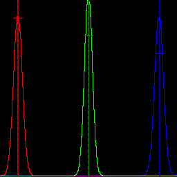
Make a sample image, and its histogram. %IMG7%magick ^ -size 200x200 xc:sRGB(10%%,50%%,90%%) ^ -attenuate 0.3 -seed 1234 +noise Gaussian ^ chst_nse_examp.jpg call %PICTBAT%histoGraph ^ chst_nse_examp.jpg chst_nse_examp_hg.png |
|
What are the SDs of the example image?
%IMG7%magick ^
  chst_nse_examp.jpg ^
  -verbose info: |grep -i deviation
@chst_nse_examp1.lis
We get one result for each of the channels, and the final number is a composite result which is the average of the channels.
An alternative for the composite is to find the SD of all the pixel values, irrespective of which channel they came from. If that is more suitable, the channels can be separated, then appended, and the statistics calculated from that image. This method will yield a larger SD.
%IMG7%magick ^
  chst_nse_examp.jpg ^
  -separate +append +repage ^
  -verbose info: |grep -i deviation
@chst_nse_examp2.lis
With this method, for this image, the combined SD is more than ten times the value of the individual channel SDs.
mean = sum_one

SD = sqrt (area/(area-1) * (sum_squared - mean * mean))

skewness = (sum_cubed - 3 * mean * sum_squared + 2 * mean^3 ) / SD^3

kurtosis = (sum_fourth - 4 * mean * sum_cubed + 6 * mean^2 * sum_squared - 3 * mean^4 ) / SD^4 - 3.0
... where:
... and so on.
To calculate the mean, the most accurate method is to sum the values and divide by the number of values, using long double data types. An alternative would be Welford's method, but that was slightly less accurate.
We calculate the other statistics (SD, skewness and kurtosis) in a single pass with Welford's method. We could use the two-pass method, using the calculated mean. This is less accurate, and takes about twice as long.
We do the calculations in data type double. Long double would give greater precision, but takes twice as long. Except for the mean calculation, double gives sufficient precision.
Statistics sum_squared, sum_cubed and sum_fourth_power are not used in MagickCore or MagickWand, but are made available in Magick++/lib/Statistic.cpp. So we need to calculate these.
When the SD is zero, the skewness and kurtosis are undefined. My code sets skewness and kurtosis to zero. (The old code would set skewness to zero, and would set kurtosis to zero or -3 or 1.3e+49 or something else.) Beware that if SD is zero for one channel (for example, alpha is fully opaque) then the overall statistics for skewness and kurtosis theoretically should not be defined.
In IM v7.1.1-20, and all previous versions I have seen, "magick ... -verbose info:" and fx.c give different results for skewness and kurtosis. The problem is in fx.c (both "-fx" and "%[fx:...]").
%IMG7%magick toes.png -colorspace Gray -auto-level -verbose info: |grep -E "deviation|skewness|kurtosis"
@chst_verbinfo.lis
The "-verbose info:" results are correct.
%IMG7%magick toes.png -colorspace Gray -auto-level -format "SD=%%[fx:standard_deviation]\nskew=%%[fx:skewness]\nkurt=%%[fx:kurtosis]\n" info:
@chst_fx.lis
The "-fx" results for skewness and kurtosis are wrong. To get the correct values, we need to multiply by QuantumRange:
%IMG7%magick toes.png -colorspace Gray -auto-level -format "SD=%%[fx:standard_deviation]\nskew=%%[fx:skewness*QuantumRange]\nkurt=%%[fx:kurtosis*QuantumRange]\n" info:
@chst_fx2.lis
This is a very old bug in fx.c. Skewness and kurtosis are dimensionless. If we multiply an image by k, the mean and standard deviation should also multiply by k, but skewness and kurtosis should not change.
I have raised this in the forum as an issue: fx calculations of skewness and kurtosis.
Suppose an image has n0 pixels value v0, and n1 pixels at value v1. The n:
mean = (n0 * v0 + n1 * v1) / (n0 + n1)

variance = (n0 * v0*v0 + n1 * v1*v1) / (n0 + n1) - mean * mean

SD = sqrt(variance)
For example, n0=100, n1 = 1000000, v0=0.1, v1 = 0.9:
mean = (100 * 0.1 + 1000000 * 0.9) / (1000100)
     = ( 10 + 9000000) / 1000100
     = 0.899920007999200079992000799920007999200079992001

variance = (n0 * v0^2 + n1 * v1^2) / (n0 + n1) - mean * mean

SD = sqrt(variance)
How do we tweak an image so its statistic become some desired values? We can make its histogram a normal distribution. So the question becomes: what transformation makes a normal distribution into a desired SD, skewness and kurtosis? The process module Set mean and stddev can teak an image to a given mean and SD, by iteration. The process module mkgauss can directly make a Gaussian distribution with given mean and SD.
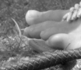
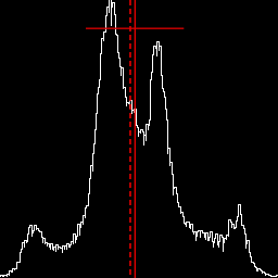
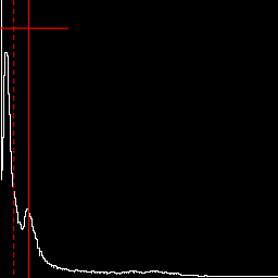
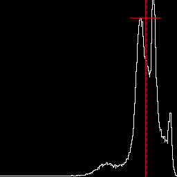
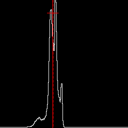
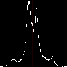
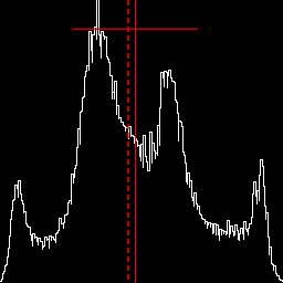
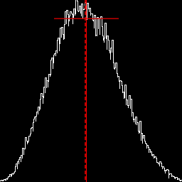
https://en.wikipedia.org/wiki/Pearson_distributionThe graph includes a vertical red line at the mean, and horizontal red lines to each side of the mean that shows the mean plus or minus one standard deviation. It also shows the median as a vertical dashed red line. The median is always within the mean plus or minus the standard deviation:
| (μ - median) | <= σ
... where |.| is the absolute operation.
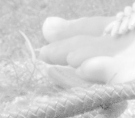
If the median is to the left of the mean, skewness is likely to be positive.
%IM7DEV%magick ^
  %SRC1% ^
  -colorspace Gray -auto-level ^
  +write chst_stats1.jpg ^
  -format "%sFMT%" ^
  info:

call %PICTBAT%histoGraph ^
  chst_stats1.jpg chst_stats1_hg.png
@chst_stats1.lis |
|
|
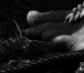
Lower mid-tones, pushing values to left of histogram, creating a positive skew. %IM7DEV%magick ^ %SRC1% ^ -colorspace Gray -auto-level ^ -evaluate Pow 4 ^ +write chst_stats2.jpg ^ -format "%sFMT%" ^ info: call %PICTBAT%histoGraph ^ chst_stats2.jpg chst_stats2_hg.png @chst_stats2.lis |
|
|
Raise mid-tones, pushing values to right of histogram, creating a negative skew. %IM7DEV%magick ^ %SRC1% ^ -colorspace Gray -auto-level ^ -evaluate Pow 0.25 ^ +write chst_stats3.jpg ^ -format "%sFMT%" ^ info: call %PICTBAT%histoGraph ^ chst_stats3.jpg chst_stats3_hg.png @chst_stats3.lis |
|
|
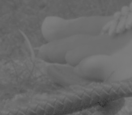
As previous, halved. This halves the mean and SD, but not skewness or kurtosis. An image with negative skew is not necessarily high-key. %IM7DEV%magick ^ %SRC1% ^ -colorspace Gray -auto-level ^ -evaluate Pow 0.25 ^ -evaluate Multiply 0.5 ^ +write chst_stats3b.jpg ^ -format "%sFMT%" ^ info: call %PICTBAT%histoGraph ^ chst_stats3b.jpg chst_stats3b_hg.png @chst_stats3b.lis |
|
|
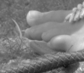
Reduce mid-tone contrast. %IM7DEV%magick ^ %SRC1% ^ -colorspace Gray -auto-level ^ +sigmoidal-contrast 5x50%% ^ +write chst_stats4.jpg ^ -format "%sFMT%" ^ info: call %PICTBAT%histoGraph ^ chst_stats4.jpg chst_stats4_hg.png @chst_stats4.lis |
|
|
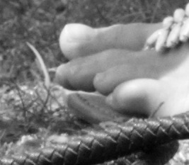
Increase mid-tone contrast. %IM7DEV%magick ^ %SRC1% ^ -colorspace Gray -auto-level ^ -sigmoidal-contrast 5x50%% ^ +write chst_stats5.jpg ^ -format "%sFMT%" ^ info: call %PICTBAT%histoGraph ^ chst_stats5.jpg chst_stats5_hg.png @chst_stats5.lis |
|
|
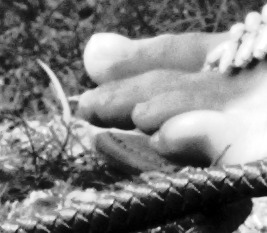
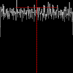
Equalize. %IM7DEV%magick ^ %SRC1% ^ -colorspace Gray -auto-level ^ -equalize ^ +write chst_stats6.jpg ^ -format "%sFMT%" ^ info: call %PICTBAT%histoGraph ^ chst_stats6.jpg chst_stats6_hg.png @chst_stats6.lis |
|
|
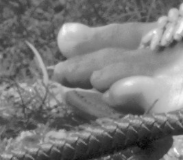
Match to a Gaussian distribution. %IM7DEV%magick ^ %SRC1% ^ -colorspace Gray -auto-level ^ chst_gray.miff call %PICTBAT%matchGauss ^ chst_gray.miff chst_stats7.miff %IM7DEV%magick ^ chst_stats7.miff ^ -colorspace Gray ^ +write chst_stats7.jpg ^ -format "%sFMT%" ^ info: call %PICTBAT%histoGraph ^ chst_stats7.jpg chst_stats7_hg.png @chst_stats7.lis |
|
For convenience, .bat scripts are also available in a single zip file. See Zipped BAT files.
rem Make a graph of histogram, showing mean, SD and median.

setlocal

set INFILE=%1
set OUTFILE=%2

for /F "usebackq" %%L in (`%IM7DEV%magick ^
  %INFILE% ^
  -format "COLSP=%%[colorspace]" ^
  info:`) do set %%L

if "%COLSP%"=="Gray" (
set sFMT=^
MNR=%%[fx:mean.r]\n^
SDR=%%[fx:standard_deviation.r]\n^
MEDR=%%[fx:median.r]\n
) else (
set sFMT=^
MNR=%%[fx:mean.r]\n^
SDR=%%[fx:standard_deviation.r]\n^
MEDR=%%[fx:median.r]\n^
MNG=%%[fx:mean.g]\n^
SDG=%%[fx:standard_deviation.g]\n^
MEDG=%%[fx:median.g]\n^
MNB=%%[fx:mean.b]\n^
SDB=%%[fx:standard_deviation.b]\n^
MEDB=%%[fx:median.b]\n
)

for /F "usebackq" %%L in (`%IM7DEV%magick ^
  %INFILE% ^
  -format "%sFMT%" ^
  +write info: ^
  +format ^
  -process 'mkhisto capnumbuckets 512 norm' ^
  %OUTFILE%`) do set %%L

call %PICTBAT%graphLineCol %OUTFILE% . . 0

if "%COLSP%"=="Gray" (
  %IMG7%magick ^
    %glcOUTFILE% ^
    -stroke Red ^
    -draw "stroke-dasharray 4,4 stroke-opacity 0.75 line %%[fx:%MEDR%*w],0,%%[fx:%MEDR%*w],%%[fx:h-1]" ^
    -draw "line %%[fx:%MNR%*w],0,%%[fx:%MNR%*w],%%[fx:h-1]" ^
    -draw "line %%[fx:(%MNR%-%SDR%)*w],%%[fx:h*0.1],%%[fx:(%MNR%+%SDR%)*w],%%[fx:h*0.1]" ^
    %OUTFILE%
) else (
  %IMG7%magick ^
    %glcOUTFILE% ^
    -stroke Red ^
    -draw "stroke-dasharray 4,4 stroke-opacity 0.75 line %%[fx:%MEDR%*w],0,%%[fx:%MEDR%*w],%%[fx:h-1]" ^
    -draw "line %%[fx:%MNR%*w],0,%%[fx:%MNR%*w],%%[fx:h-1]" ^
    -draw "line %%[fx:(%MNR%-%SDR%)*w],%%[fx:h*0.1],%%[fx:(%MNR%+%SDR%)*w],%%[fx:h*0.1]" ^
    -stroke Green ^
    -draw "stroke-dasharray 4,4 stroke-opacity 0.75 line %%[fx:%MEDG%*w],0,%%[fx:%MEDG%*w],%%[fx:h-1]" ^
    -draw "line %%[fx:%MNG%*w],0,%%[fx:%MNG%*w],%%[fx:h-1]" ^
    -draw "line %%[fx:(%MNG%-%SDG%)*w],%%[fx:h*0.2],%%[fx:(%MNG%+%SDG%)*w],%%[fx:h*0.2]" ^
    -stroke Blue ^
    -draw "stroke-dasharray 4,4 stroke-opacity 0.75 line %%[fx:%MEDB%*w],0,%%[fx:%MEDB%*w],%%[fx:h-1]" ^
    -draw "line %%[fx:%MNB%*w],0,%%[fx:%MNB%*w],%%[fx:h-1]" ^
    -draw "line %%[fx:(%MNB%-%SDB%)*w],%%[fx:h*0.3],%%[fx:(%MNB%+%SDB%)*w],%%[fx:h*0.3]" ^
    %OUTFILE%
)
rem Root finder: finds value of PP for which expression is roughly zero.
rem %1 expression that contains PP
rem %2 prefix for output environment variables
rem %3 lower guess for PP
rem %4 upper guess for PP
rem %5 epsilon for convergence
@rem
@rem If there is a value of PP between the guesses for which the expression is zero,
@rem this should find it.
@rem
@rem There may be more than one root, but this will find only one.
@rem
@rem Evaluating the expression for the two guesses should give opposite signs,
@rem so the zero crossing is between the guesses.
@rem If that isn't true, the fx expression will write a debug line like:
@rem   [0,0].[64]: Err=1
@rem Even if an error is raised, it may still find a correct solution.
@rem
@rem The code also emits Vmid, the value of the expression at the returned value of PP.
@rem A caller can consider whether the value is close enough to zero.

setlocal

set EXP=%~1
if "%EXP%"=="." set EXP=
if "%EXP%"=="" set EXP=PP*log(PP) + log(1-PP) - PP*log(1-PP) + 0.5*log(2)

set EnvPref=%2
if "%EnvPref%"=="." set EnvPref=

set Guess1=%3
if "%Guess1%"=="." set Guess1=
if "%Guess1%"=="" set Guess1=0

set Guess2=%4
if "%Guess2%"=="." set Guess2=
if "%Guess2%"=="" set Guess2=1

set Eps=%5
if "%Eps%"=="." set Eps=
if "%Eps%"=="" set Eps=1e-9

set fxSolve=^
Pone=%Guess1%; ^
Ptwo=%Guess2%; ^
Warn=0; ^
while (abs(Pone-Ptwo)^>%Eps%, ^
  PP=Pone; ^
  Vone=%EXP%; ^
  PP=Ptwo; ^
  Vtwo=%EXP%; ^
  if (sign(Vone)==sign(Vtwo),Warn=1, ); ^
  PP=(Pone + Ptwo)/2; ^
  Vmid=%EXP%; ^
  if (sign(Vmid)==sign(Vone),Pone=PP,Ptwo=PP) ^
); ^
if (Warn==1, debug(Warn), ); ^
debug(Vmid); ^
PP


for /F "usebackq tokens=1,2,* delims== " %%A in (`%IMG7%magick ^
  xc: ^
  -precision 15 ^
  -format "%%[fx:%fxSolve%]" ^
  info: 2^>^&1`) do (
  echo A=%%A B=%%B C=%%C
  if "%%B"=="Vmid" (
    set Vmid=%%C
  ) else (
    set PP=%%A
  )
)

echo Vmid=%Vmid%
echo PP=%PP%

endlocal & set %EnvPref%_Vmid=%Vmid%& set %EnvPref%_PP=%PP%
All images on this page were created by the commands shown, using:
%IMG7%magick -version
Version: ImageMagick 7.1.1-20 Q16-HDRI x86 98bb1d4:20231008 https://imagemagick.org
Copyright: (C) 1999 ImageMagick Studio LLC
License: https://imagemagick.org/script/license.php
Features: Cipher DPC HDRI OpenCL OpenMP(2.0)
Delegates (built-in): bzlib cairo freetype gslib heic jng jp2 jpeg jxl lcms lqr lzma openexr pangocairo png ps raqm raw rsvg tiff webp xml zip zlib
Compiler: Visual Studio 2022 (193532217)
To improve internet download speeds, some images may have been automatically converted (by ImageMagick, of course) from PNG or TIFF or MIFF to JPG.
Source file for this web page is chstat.h1. To re-create this web page, execute "procH1 chstat".
This page, including the images, is my copyright. Anyone is permitted to use or adapt any of the code, scripts or images for any purpose, including commercial use.
Anyone is permitted to re-publish this page, but only for non-commercial use.
Anyone is permitted to link to this page, including for commercial use.
Page version v1.0 8-December-2023.
Page created 01-Mar-2024 15:13:09.
Copyright © 2024 Alan Gibson.